Nutrients Mini Experiment (Part 1)
This week I have made some progress using the idealized estuary to compare bottom DO with and without nutrients in WWTP effluent. There is more analysis work I can do later on, and I have some questions about my boundary conditions. However, I wanted to document and share the current experiment status prior to my trip.
For this experiment, I have been using the grid I developed when writing the WWTP placement algorithm (documentation in prior blog post). As a reminder, Figure 1 shows the model grid and locations of point sources.
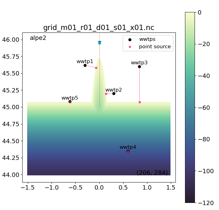
Fig 1. Grid bathymetry and point source locations. Note that this grid also includes a river.
I let the model run for two months to spin-up without DIN in the WWTP effluent. Then, I ran the model for one additional month under two conditions: (1) the base case in which I let the model continue with no DIN in the WWTP effluent; and (2) the nutrient condition in which I added DIN to the WWTP effluent.
More details about the initial conditions, model spin-up, preliminary results, and boundary conditions are provided below.
Model Spin-Up Initial Conditions
I used four types of forcing during the model spin-up: ocean, atmospheric, tidal, and river forcing. The river forcing includes forcing conditions for both the river and WWTPs.
Ocean Forcing
The values used for ocean forcing are listed below. With the exception of salinity, the ocean forcing variables are constants.
The value of non-listed variables is zero (e.g. free surface height or ammonium concentration).
| Variable | Description | Value | Notes |
|---|---|---|---|
| salt | ocean salinity | 30 g kg-1 (ocean) 0 g kg-1 (estuary) |
Estuary half fresh at t = 0. IC shown in Fig 2. |
| temp | sea water temperature | 10 C | Same as air, river, and WWTP effluent temp |
| NO3 | nitrate concentration | 27 mmol N m-3 | Salish Sea IC in ocn1/Ofun_bio |
| phytoplankton | conc of phytoplankton as N | 0.1 mmol N m-3 | Some small amount to start |
| zooplankton | conc of zooplankton as N | 0.1 mmol N m-3 | Some small amount to start |
| TIC | conc of total inorganic C | 2037 mmol C m-3 | Salish Sea IC in ocn1/Ofun_bio |
| alkalinity | total alkalinity | 2077 milliequivalent m-3 | Salish Sea IC in ocn1/Ofun_bio |
| oxygen | conc of DO | 219 mmol O m-3 (7 mg L-1) |
Salish Sea IC in ocn1/Ofun_bio |
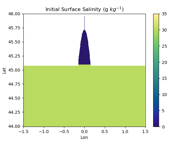
Fig 2. Ocean salinity initial condition.
Atmospheric Forcing
All atmospheric forcing state variables are listed below. All values are constat, except for shortwave radiation which has a daily cycle shown in Figure 3.
| Variable | Description | Value | Notes |
|---|---|---|---|
| Pair | air pressure | 1013.25 mbar | |
| rain | rainfall rate | 0 kg m2 s-1 | |
| swrad | shortwave radiation | daily cycle with peak of 500 W m-2 | Hourly profile shown in Fig 3. |
| lwrad_down | downwelling longwave radiation | 290 W m-2 | |
| Tair | air temperature | 10 C | Same as ocean, river, and WWTP effluent temp |
| Qair | relative humidity | 83% | |
| Uwind | E-W wind speed | 0 m s-1 | |
| Vwind | N-S wind speed | 0 m s-1 |

Fig 3. Hourly shortwave radiation.
Tidal Forcing
Tidal forcing is made up of a simple spring-neap cycle with a solar and a lunar component.
| Variable | Description | Value |
|---|---|---|
| tide_Eamp | tidal elevation amplitude | 0.75 m (M2) 0.25 m (S2) |
| tide_period | tidal period | 12.42 hrs (M2) 12 hrs (S2) |
River/WWTP Forcing
River forcing includes both the river component and the WWTP component. The river and WWTP forcing differ from each other, but all 5 WWTPs have the same forcing.
Again, any variable that is not listed has an initial value of zero (such as small detritus).
For these forcing conditions, I borrowed several average values for the Skagit River and West Point treatment plant from Ecology’s dataset. This way, the forcing conditions will hopefully be somewhat realistic.
River Forcing
| Variable | Description | Value | Notes |
|---|---|---|---|
| river_Vshape | vertical profile | 1/N in each layer | transport evenly split between sigma layers |
| river_transport | volume transport | 1000 m3 s-1 | |
| river_salt | river salinity | 0 g kg-1 | |
| river_temp | river temperature | 10 C | Same as ocean, air, and WWTP effluent temp |
| river_NO3 | conc of nitrate | 6.4 mmol N m-3 | Average value from Skagit River (Ecology’s dataset) |
| river_TIC | conc of total inorganic C | 455 mmol C m-3 | Average value from Skagit River (Ecology’s dataset) |
| river_TAlk | total alkalinity | 410 milliequivalents m-3 | Average value from Skagit River (Ecology’s dataset) |
| river_Oxyg | conc of DO | 362 mmol O m-3 (11.6 mg L-1) |
Average value from Skagit River (Ecology’s dataset) |
WWTP Forcing
| Variable | Description | Value | Notes |
|---|---|---|---|
| river_Vshape | vertical profile | 1 in bottom layer 0 in other layers |
discharging to bottom layer |
| river_transport | volume transport | 4.5 m3 s-1 | Average value from West Point (Ecology’s dataset) |
| river_salt | river salinity | 0 g kg-1 | |
| river_temp | river temperature | 10 C | Same as ocean, air, and river temp |
| river_NO3 | conc of nitrate | 0 mmol N m-3 | Start with no nutrients for model spin-up |
| river_TIC | conc of total inorganic C | 2639 mmol C m-3 | Average value from West Point (Ecology’s dataset) |
| river_TAlk | total alkalinity | 2000 milliequivalents m-3 | Average value from West Point (Ecology’s dataset) |
| river_Oxyg | conc of DO | 184 mmol O m-3 (5.9 mg L-1) |
Average value from West Point (Ecology’s dataset) |
Model Spin-Up Results
The video below shows the daily surface temperature and salinity from the 2-month model spin-up run.
The next video shows the daily surface phytoplankton and bottom DO from the 2-month model spin-up run.
The phytoplankton grow very quickly during the first two weeks, and then suddenly dissappear (I am guessing due to a zooplankton population boom). Afterwards, the phytoplankton concentration is low and remains quite low. After the mass phytoplankton die-off, a large hypoxic region develops away from the coast. Near the coast, the river appears to introduce oxygen to the water. There also appears to be more oxygen near the WWTP locations.
Forcing for Experimental Conditions
As mentioned earlier, I ran two experimental conditions for one month using the spin-up results above.
The first condtion is the base case, and is really just a continuation of the spin-up set up. Nothing was changed in the forcing files.
The second condition is the nutrient condition. In this case, I changed the concentration of nitrate in the WWTP effluent from 0 to 344 mmol N m-3. Again, this value is the average nitrate concentration for West Point treatment plant reported in Ecology’s dataset. No other values were changed in the forcing files.
Preliminary Results
Base Case: No Nutrients in WWTP Effluent
Below is a daily movie of surface phytoplankton and bottom DO for the base case. In general, new phytoplankton are only growing near the river. The concentration of phytoplankton in the ocean is roughly zero, and new phytoplankton do not appear to grow in the ocean.
Nutrient Condition: DIN in WWTP Effluent
The video below shows the surface phytoplankton and bottom DO for the nutrient condition. This video looks very similar to the one above, except that there are more phytoplankton growing near the coastal WWTPs.
Comparison
As a preliminary comparison method, I took a look at the final hour of this model run.
Figure 4 compares the final hour surface phytoplankton from both model runs.
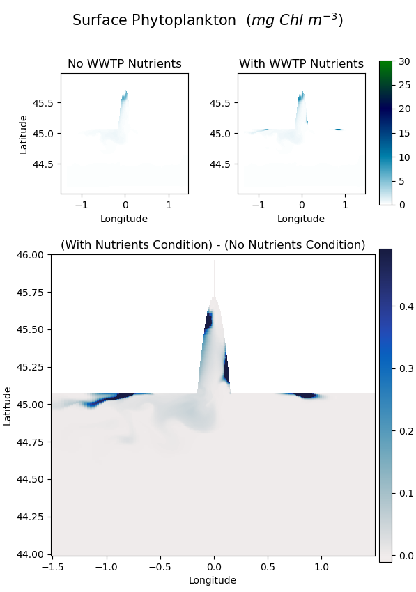
Fig 4. Final hour comparison of surface phytoplankton.
Figure 5 compares the final hour bottom DO from both model runs.
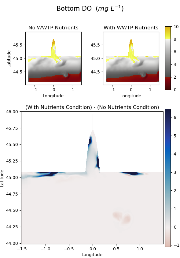
Fig 5. Final hour comparison of bottom DO.
In general, the with-nutrients conditions has more phytoplankton near the point sources than the no-nutrient base case.
The with-nutrients condition also appears to have a higher bottom DO concentration near the coastal WWTPs than the no-nutrient base case. This may be due to more phytoplankton growing near the WWTPs and producing more oxygen.
I am slightly confused why there is less oxygen near the in-ocean WWTP. There does not appear to be much phytoplankton growing near this WWTP.
My best guess for what may be going on is that near the in-ocean WWTP, the WWTP enables some phytoplankton to grow from the very small model spin-up phytoplankton population. Because the new growth has a relatively low concentration, it gets consumed and dies off quickly. The lower DO in this area is thus the result of these additional phytoplankton decomposing. In contrast, the coastal WWTPs have a larger initial phytoplankton population to grow from. Additionally, the water depth is shallower near the coast, so nitrate may be more readily available for uptake at the surface. Because of this, more phytoplankton may be growing than dying near the coastal WWTPs. This could explain why bottom DO concentration is actually greater near the coastal WWTPs in the with-nutrients case. I am curious if I let the model run for longer whether these near-coast phytoplankton populations will eventually contribute to lower bottom DO concentrations as well.
Nevertheless, my explanations remain speculative for now. I am looking forward to exploring these questions further in additional idealized model analyses or using LiveOcean!
Boundary Condition Questions
For all biogeochemistry state variables, I applied the Gradient boundary condition to the open boundaries. This means that the gradient of the variable is zero at the boundary, and the inflowing value is thus equal to the nearest within-domain value.
I am concerned that this may not be the most appropriate boundary condition for this model run. In particular, once all of the phytoplankton dies off and nitrate gets used up along the boundary, no more nutrients will be introduced from the ocean and no more phytoplankton can grow. I am guessing this is a large reason why very few phytoplankton seem to grow near the WWTP located in the ocean. Maybe it would be better to allow more nutrients and phytoplankton enter the domain from the ocean.