Bit-reproducibility issues
This week I spent more time investigating bit-reproducibility in the biogeochemistry fields. My main findings are summarized below:
- There are no bit-reproducibility issues between two identical runs
- Runs with different biogeochemical forcing still have bit-reproducible hydrodynamics (u,v,w,salt,temp)
- Runs with different biogeochemical forcing appear to have noise in the biogeochemical fields
- The noise appears in both average and history files after one day of run time
It is good to know that two identical runs do not appear to have bit-reproducibility issues. However, this also presents a problem for debugging because it will be difficult to distinguish between a true signal and unwanted noise. How will we know whether differences between two runs are due to differences in forcing or due to bit-reproducibility issues?
Experimental Set-up
To address the signal-to-noise issue, I simplified my test case. In this blog post, I compare the following two runs:
- A run with existing nutrient loads from all WWTPs
- Same as run 1, except West Point nutrients concentrations are set to zero
These new runs reduce complexity by applying forcing changes to a single grid cell location (West Point) rather than at 87 different WWTP locations.
I compared model differences after one day of run time, and verified that ocean_his_0002 and ocean_avg_0001 show similar results.
More Details
I looked at many different figures, but have only included a few key plots in this blog post.
Last week we discussed that it is important to consider differences in the model fields at different sigma-levels, rather than just the surface and bottom. This is especially true for w.
Rather than plotting a difference map at a specified sigma-level, I instead generated a two-tone map that plots binary values. Blue means that there are no differences between two model runs at any sigma-level. Black means that there are differences between the two model runs at some sigma level. We don’t know at which sigma level(s) the differences occur, nor do we know how large the differences are. We only know that there are differences at that lat/lon location. Though we lose some information, this binary plot makes it easier to see whether differences are present, and where these differences are located.
Figure 1 shows an example of a binary plot. This figure compares NH4 fields between a run with and without nutrient loads from West Point WWTP. The location of West Point is denoted by a pink circle.
For comparison, Figure 2 shows a map of the surface and bottom differences in NH4. Note that in Figure 2, our visualization of model differences is highly dependent on our choice of color bar limits. Figure 1, however, will always show us where the differences occur.
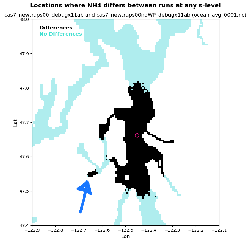
Fig 1. Locations where NH4 differs between a model run with West Point and a model run without West Point. Black indicates that there are differences, and blue indicates that there are no differences. The pink circle denotes the location of West Point WWTP.
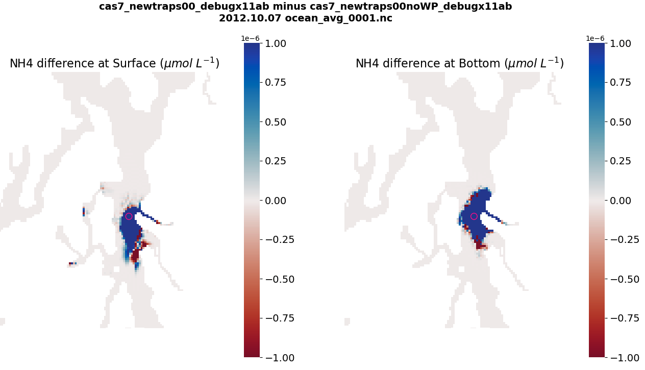
Fig 2. Comparison of NH4 concentration after one day of run time between the two runs (West Point minus no-West Point). The left panel shows surface differences. The right panel shows bottom differences. The pink circle denotes the location of West Point WWTP.
In Figure 1, I drew a blue arrow pointing to differences that appear in Sinclair Inlet. If these differences were due to the presence/absence of nutrients at West Point, then I would expect there to be a continuously propagating signal of differences between West Point and Sinclair Inlet. However, the differences in Sinclair Inlet appear to develop spontaneously. Thus, they likely signal bit-reproducibility issues.
The main takeway from my West Point experiment is that it is hard to discern what is signal and what is noise. However, I am relatively confident that we do indeed have a bit-reproducibility problem in the biogeochemistry fields.