Twin Variable Dye Experiments
Over the last few days I have conducted numerous dye experiments, and have come to the conclusion that twin variables will not eliminate our noise issue.
This blog post summarizes the experiments that led me to this conclusion. It also provides some insight into a new hypothesis: bit-precision is the true problem.
Note that all of the experiments described in this blog post involve a point-source release of dye from West Point WWTP.
The original problem
Our original noise issue popped up during Jilian’s alkalinity enhancement experiments and my WWTP loading/no-loading experiments. When we took the difference between two model runs with different forcing inputs, we observed noise in the difference field. Figure 1 is a reminder of what the difference in NH4 looked like after one day of run time, comparing a run with normal NH4 discharge from West Point WWTP to a run with no NH4 discharge from West Point.
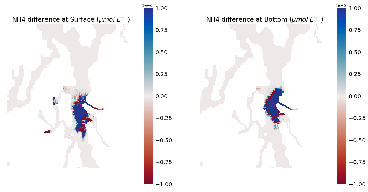
Fig 1. Comparison of NH4 concentration after one day of run time between the two runs (West Point minus no-West Point). The left panel shows surface differences. The right panel shows bottom differences. The pink circle denotes the location of West Point WWTP.
We can also visualize noise through residual plots, which show the difference in concentration vs. distance from West Point (Figure 2).
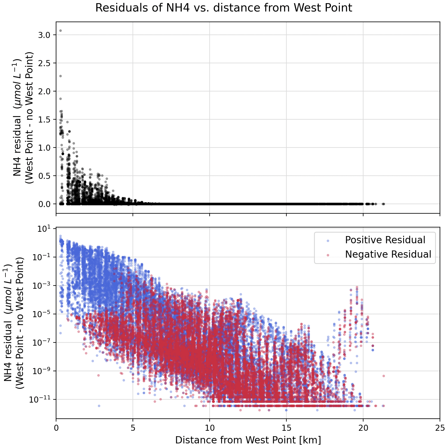
Fig 2. Residuals of NH4 (i.e. With West Point run minus no West Point run). Top panel is in linear scale, bottom panel is in log scale, with positive residuals colored in blue and negative residuals colored in red.
Throughout this blog post, I will describe my modeling experiments using schematics. Figure 3 shows the schematic corresponding to my original loading/no-loading experiment.
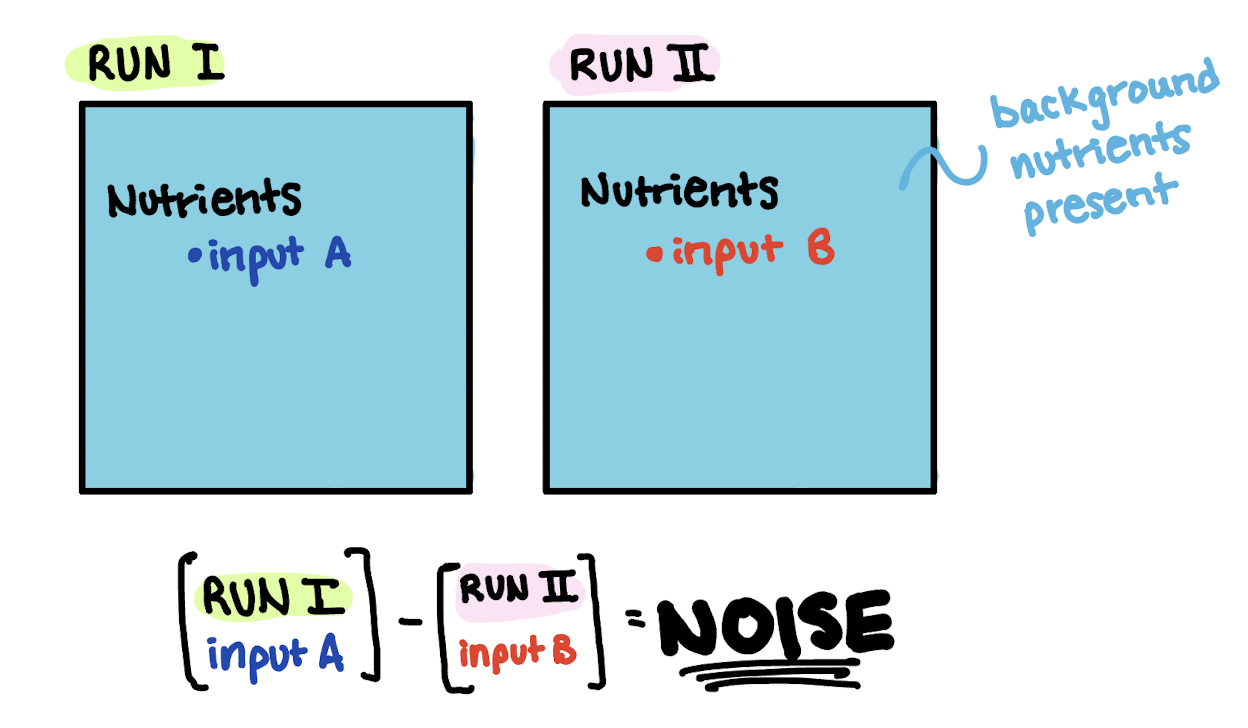
Fig 3. Schematic of original loading/no-loading experiment.
Each square in the schematic represents a different model run, labeled “Run I” or “Run II”. Within the model run, there is a variable of “Nutrients.” Their forcing inputs are labeled “input A” in Run I and “input B” in Run II to indicate that the forcing inputs are different across the runs. The blue background indicates that there are background nutrient concentrations in the model ocean field.
The equation below the schematic shows how we calculated differences. In this case, we compared the difference between the two model runs which had different forcing inputs, and we obtained a noisy result.
One exponentially decaying dye
The first test I ran helped confirm that I correctly implemented exponentially decaying dye.
I ran a single model run with zero background dye concentration, but had a single point source of dye at West Point WWTP. This model run contains two dyes: dye_01 which behaves as an inert passive tracer, and dye_02 which decays exponentially. They discharge at the same concentration from West Point (Figure 4).
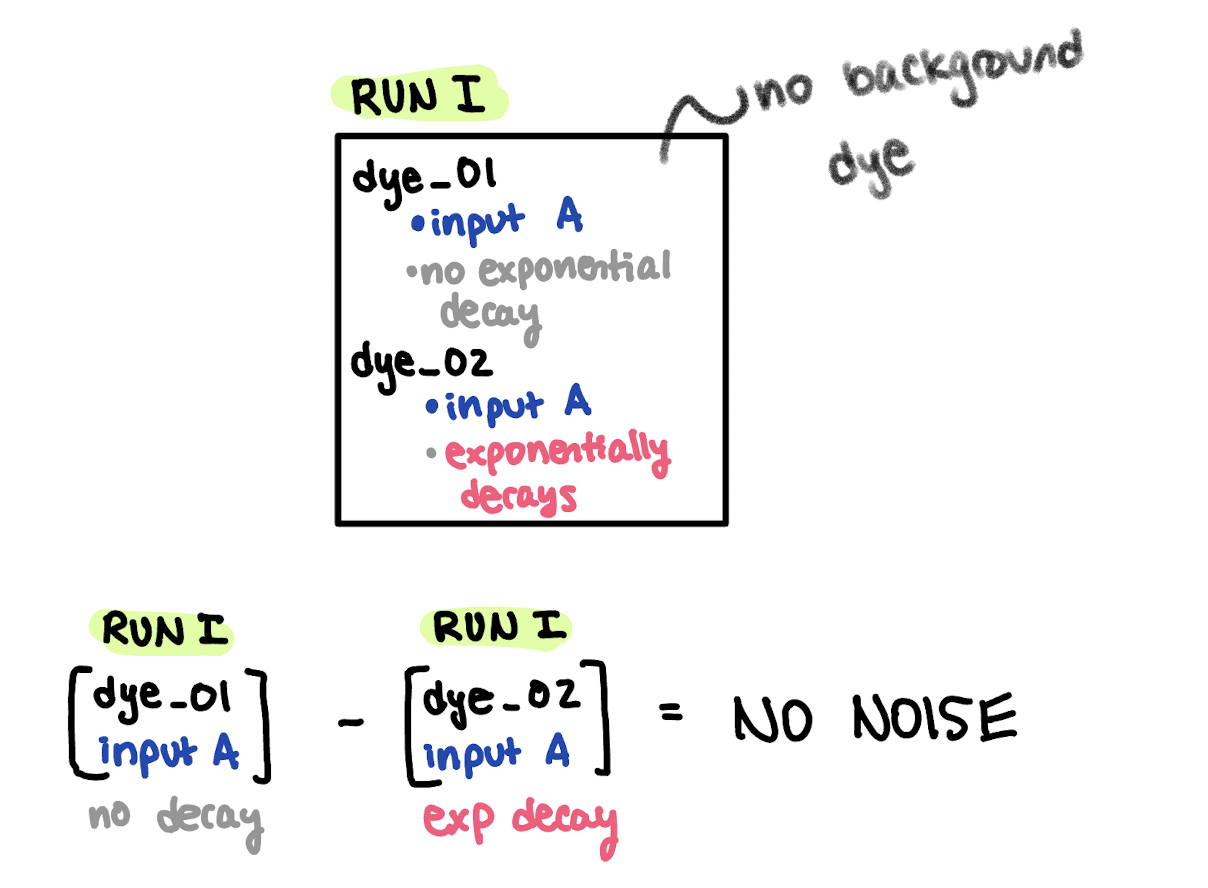
Fig 4. Schematic of experiment to verify exponentially decaying dye behaves correctly.
The video below shows the difference in concentration between dye_01 and dye_02 over one day of run time (Figure 5). There is no apparent noise in this run, which we can confirm using residual plots (Figure 6). The residuals are generally always positive, suggesting that dye_01 is always greater than dye_02, which is what we would expect!
Fig. 5 Dye release test from West Point WWTP. Every frame corresponds to an hourly snapshot, and the video spans one day. Discharge concentration was 10 kg/m3 of dye.
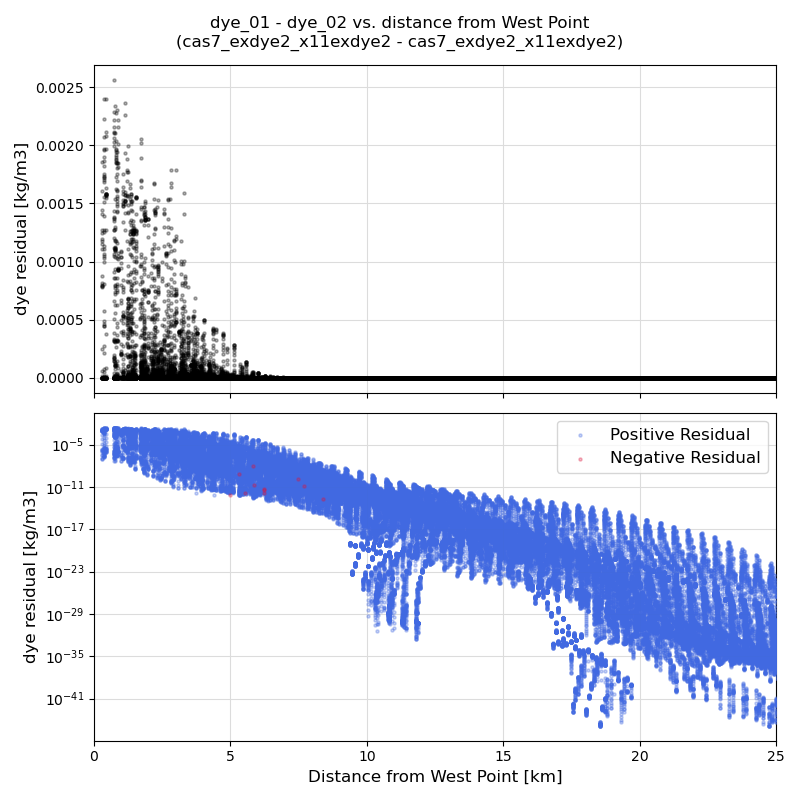
Fig 6. Residuals of dye. Top panel is in linear scale, bottom panel is in log scale, with positive residuals colored in blue and negative residuals colored in red.
Lastly, I verified that dye_02 correctly decays exponentially. I know the discharge rate and concentration from West Point WWTP, and I know the exponential decay rate of dye, so I should be able to predict the total integrated mass of dye_01 and dye_02 in the model domain for all time. Figure 7 shows the analytically predicted dye mass (lines) compared to the modeled dye mass (dots). Since everything lines up, we can confirm that we implemented exponential decay correctly!
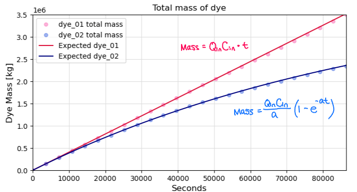
Fig 7. Total modeled and analytically predicted mass of dye in the LiveOcean domain. Qin is the discharge rate from West Point WWTP (4 m3/s). Cin is the discharge concentration (10 kg/m3 for both dye_01 and dye_02). a is the exponential decay rate (1e-5 1/s).
Hypothesis 1: Noise is inherent to running two separate simulations
Next, I ran two identical model runs. They both have equal discharge concentrations of dye_01 and dye_02 from West Point WWTP. dye_01 is an inert passive tracer, and dye_02 decays exponentially. There is no background concentration of dye. Figure 8 shows the schematic for this experiment.
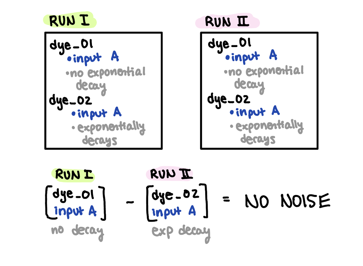
Fig 8. Schematic of experiment to test whether noise is inherent to two different model runs.
I compared dye_01 from Run 1 to dye_02 in Run II, and found no noise in the results. The results are identical to those from the previous section of this blog. Thus, noise is not inherent to running two separate simulations.
Hypothesis 2: Noise is caused by differences in forcing in two different model runs
Next, I altered dye_01 so that it also behaves as an exponentially decaying dye. dye_01 and dye_02 have the same decay rate, therefore we can consider them to be identical tracers, i.e twin variables.
We observed noise in the original loading/no-loading experiment when we changed the input forcing between runs. Thus, I test the hypothesis that differences in forcing between model runs is the source of the noise.
I ran two identical simulations with twin variables dye_01 and dye_02 that both decay exponentially. However, dye_01 has a different discharge concentration from West Point WWTP compared to dye_02 (Figure 9).
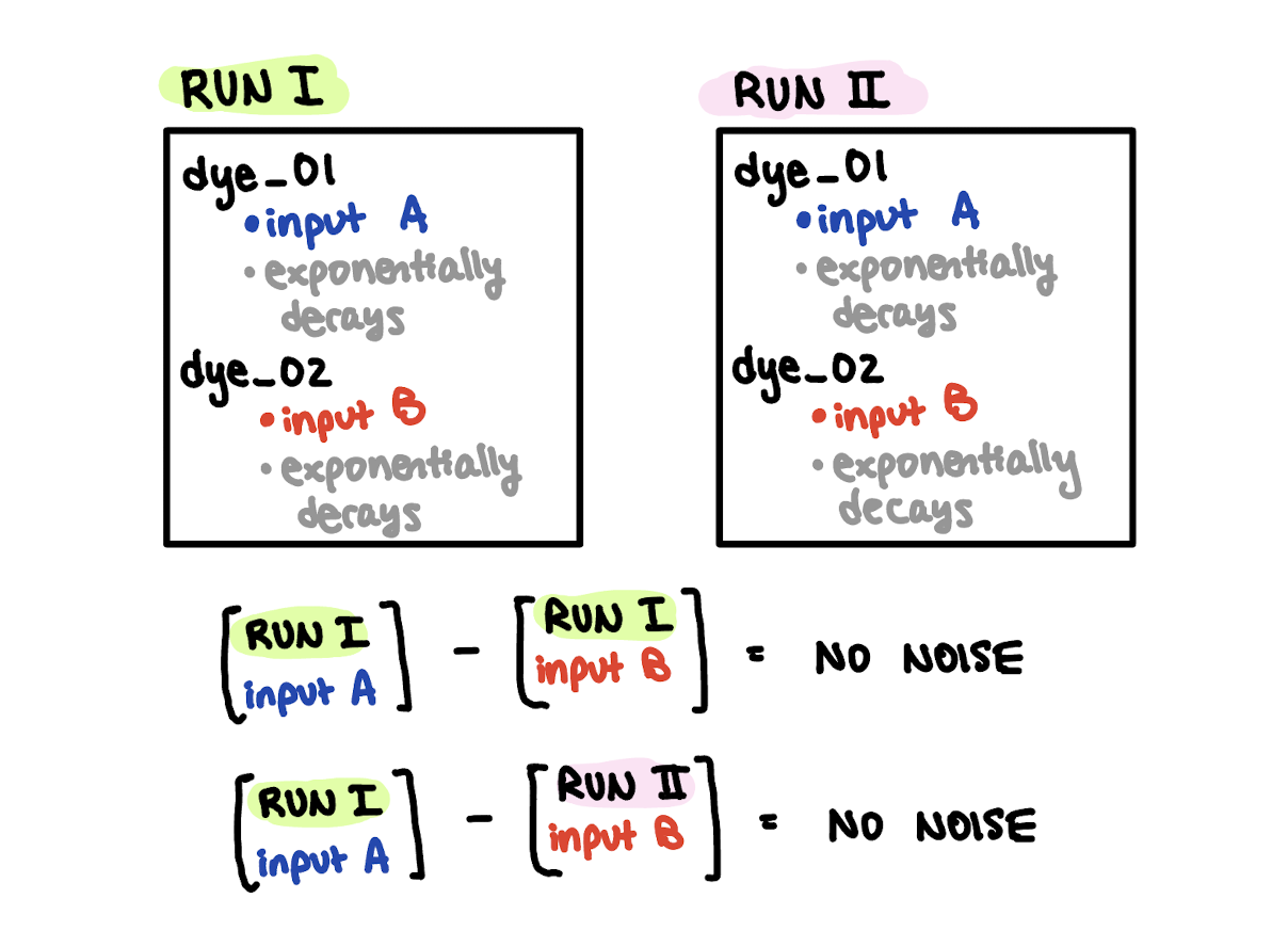
Fig 9. Schematic of experiment to test whether noise is generated by differences in forcing inputs across two different model runs.
I hypothesized that the difference between dye_01 and dye_02 across the two different runs would generate noise, but the difference within the same run would not generate noise. However, neither case generated noise.
Hypothesis 3: Noise is caused by interactions with background concentrations
In the original loading/no-loading experiment, there were background concentrations of nutrients in the water. Therefore, my next hypothesis was that noise is caused by interactions of the tracer with background concentrations.
I set up a repeat experiment as the previous section, but I added a constant background dye_01 and dye_02 concentration of 0.1 kg/m3 (Figure 10).
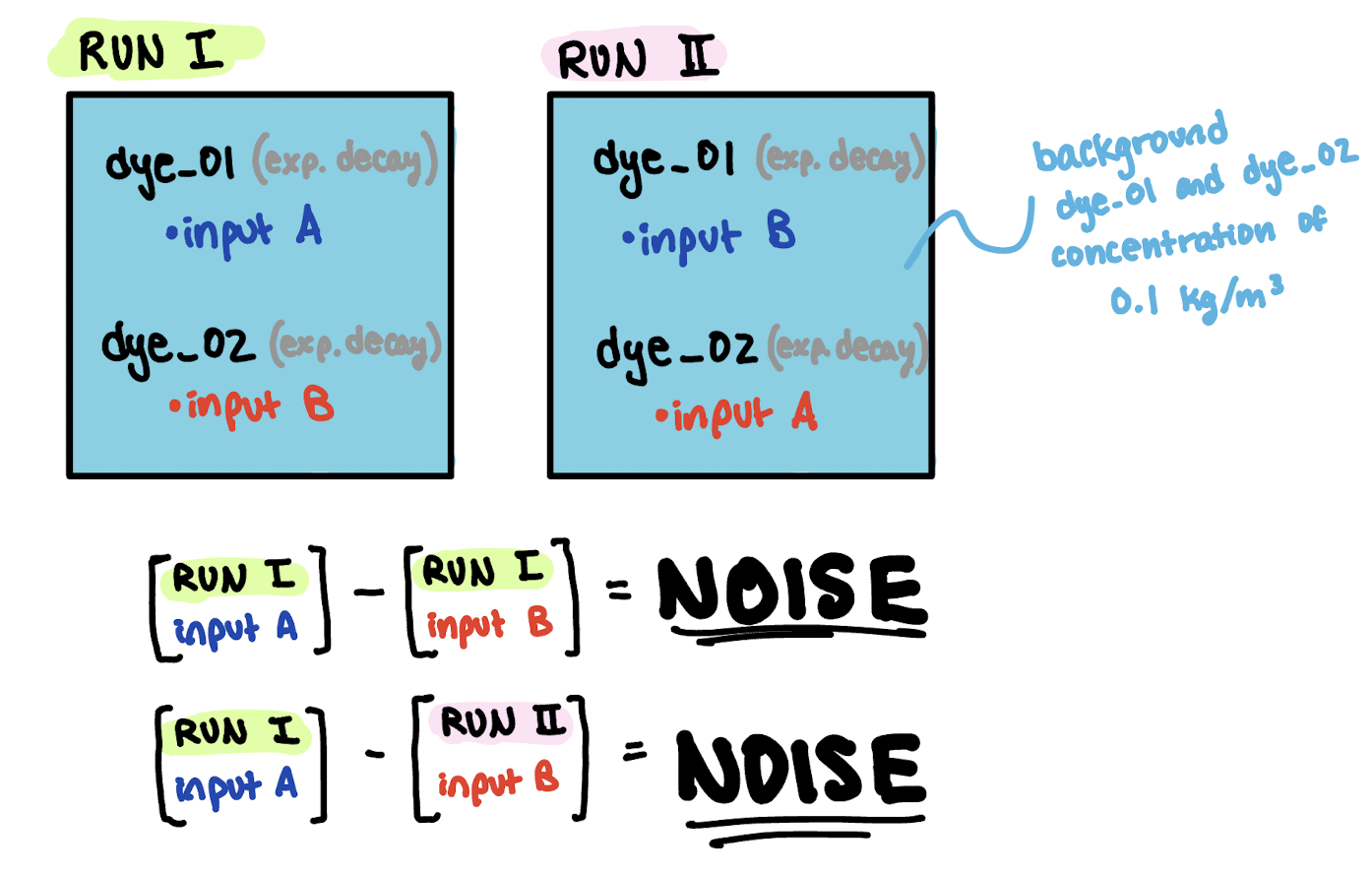
Fig 10. Schematic of experiment to test whether noise is generated by interactions between tracer and background concentrations.
I hypothesized that the difference between dye_01 and dye_02 across the two different runs would generate noise as it interacted with the background dye concentrations, but the difference within the same run would not generate noise. Surprisingly, both tests resulted in noise, and they were both equally noisy!
Figure 11 shows the evolution of the difference in dye concentrations over the course of one day, and Figure 12 shows the residuals at the end of one day. Noise is present in both visualizations.
Fig. 11 Dye release test from West Point WWTP. Every frame corresponds to an hourly snapshot, and the video spans one day. Discharge concentration was 10 kg/m3 for dye_01, and 5 kg/m3 for dye_02. Both decay exponentially, and they behave as twin variables. There is an initial background dye cocentration of 0.1 kg/m3 everywhere.
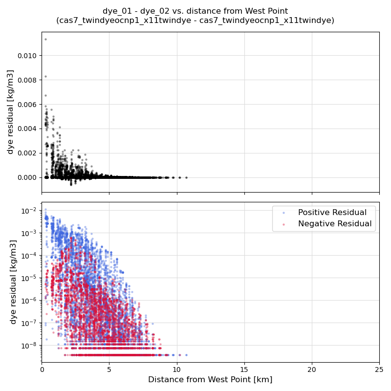
Fig 12. Residuals of dye. Top panel is in linear scale, bottom panel is in log scale, with positive residuals colored in blue and negative residuals colored in red.
These results suggest that noise is generated by the presence of a background concentration of tracer, and that twin variables will not resolve the issue.
Hypothesis 4: Noise is related to bit-precision and significant figures
My latest hypothesis is that noise is related to the bit-precision of the model and the amount of significant figures it can carry around.
To illustrate, let’s assume that the model can only store 7 significant figures. If we have zero background dye concentration, then all 7 significant figures are able to capture the tiny differences due to our tiny forcing input changes (because the most significant bit is a tiny number). However, if the background concentration of dye is large, then these 7 significant figures begin at a larger value, and are thus unable to resolve the tiny differences due to our forcing changes.
To test this hypothesis, I ran an identical experiment as the previous section, but I decreased the background dye concentration from 0.1 kg/m3 to 1e-6 kg/m3 (Figure 13).
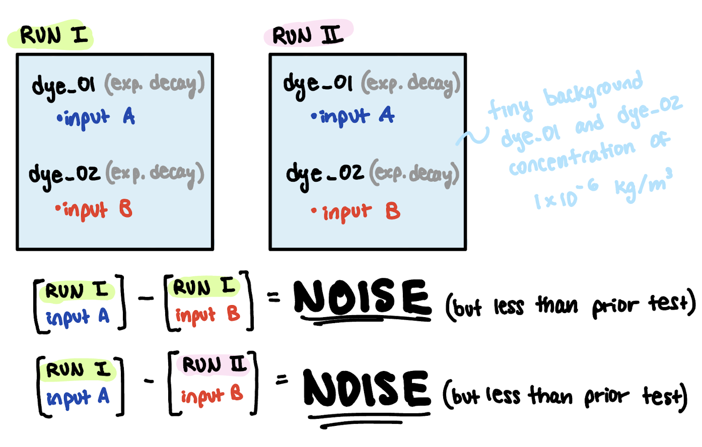
Fig 13. Schematic of experiment to test whether noise is generated by bit-precision and limitations on significant figures.
I still observed noise in this test. However, the noise appears less extreme compared to when the background concentrations were large (Figures 14 and 15). Note that the y-scale of the residual plot is different than in the previous plot (sorry!).
Fig. 14 Dye release test from West Point WWTP. Every frame corresponds to an hourly snapshot, and the video spans one day. Discharge concentration was 10 kg/m3 for dye_01, and 5 kg/m3 for dye_02. Both decay exponentially, and they behave as twin variables. There is an initial background dye cocentration of 1e-6 kg/m3 everywhere.
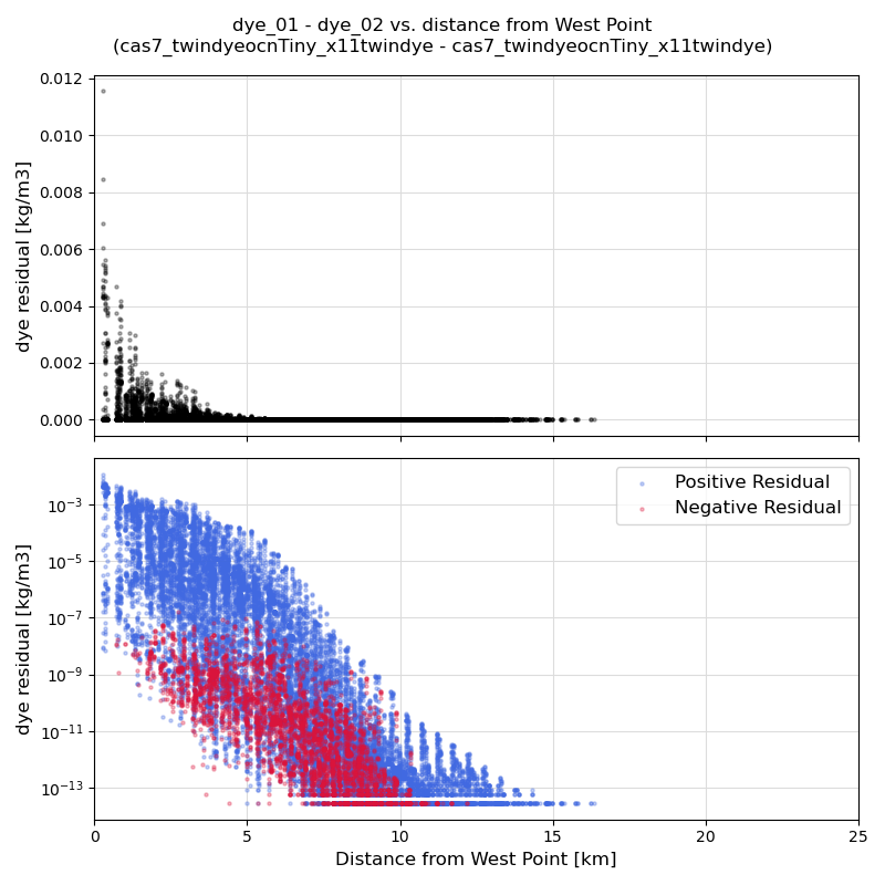
Fig 15. Residuals of dye. Top panel is in linear scale, bottom panel is in log scale, with positive residuals colored in blue and negative residuals colored in red.
Conclusion
Twin variables won’t resolve the noise issue. My current working hypothesis is that noise is related to the amount of bit-precision available to resolve significant figures.