Noise Evolution
At the time of writing, my no-loading simulation has run for over one year. This week I took a look at noise using the normalized integral approach of total nitrogen that Parker recommended. More details below.
Based on the results, I think the noise is small relative to the signal in Puget Sound, which is good for our WWTP loading experiment. However, boundary noise can be relatively large, and may be problematic for future mCDR experiments conducted across the whole domain.
Description of figure
Previously, Parker had developed a method for investigating noise using a pcolormesh plot of normalized vertical integrals of total nitrogen. Last week, Alex recommended that I look at noise at the boundaries, and Kate recommended that I sum up noise within a domain and plot the noise evolution with time.
I combined all of these suggestions into one video, and I apologize because the result is a rather complicated concoction.
Figure 1 shows a single frame of the videos below. There are three components to this figure: (1) the pcolormesh, (2) the bottom panel, and (3) the right panel.
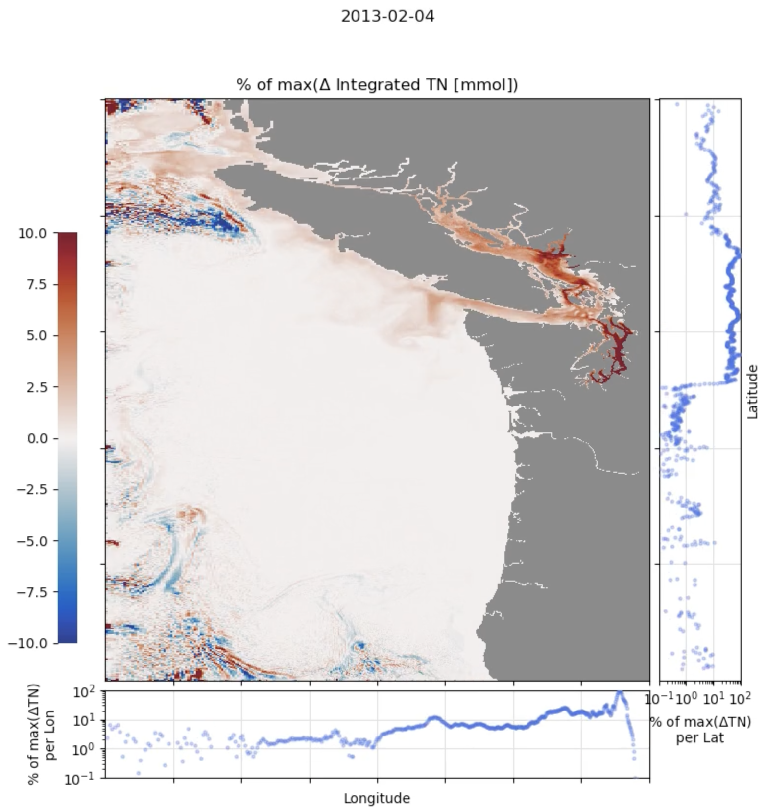
Fig 1. Single frame snapshot of the type of figure I used to evaluate noise in the WWTP loading experiment.
pcolormesh
The pcolormesh is very similar to the figures that Parker shared with us before. I started with his code, and adapted it from there. The data processing steps taken to create this pcolormesh panel were:
- Sum all of the constituents in the NPZD module (NO3, NH4, phytoplankton, zooplankton, large & small detritus) to obtain total nitrogen (TN) in each grid cell
- Vertically integrate TN at every grid cell in the model domain
- Multiply vertical integrals of TN by the horizontal area of each grid cell to obtain TN in mmol at every lat/lon location in the model domain.
- Calculate the difference in TN [mmol] between the “loading” run and the “no-loading” run at every lat/lon location of the model domain
- Normalize the colorbar scale by dividing by the maximum difference in TN [mmol] between the two runs (i.e., the largest signal)
The result is a pcolormesh map where the color represents the size of the difference in TN between the two model runs relative to the location where there is the largest difference in TN between the two runs.
The colorbar limits span from -10% to 10%.
bottom panel
The bottom panel chunks the data into columns, based on longitude. I took the difference in TN between the two model runs (i.e., the results from Step 4 of the pcolormesh plot), and I summed that difference within columns of constant longitude. Then, I normalized the results by dividing by the maximum longitude sum of the difference in TN [mmol] between the two runs.
The resulting figure shows longitude on the x-axis (which aligns exactly to the longitude on the pcolormesh panel), and the normalized sum of differences within a line of longitude relative to the maximum sum of differences within a line of longitude.
Note that the y-axis is in log scale and spans from 0.1% to 100%. I also took the absolute value of the differences, and plotted positive differences in blue and negative differences in red– though it seems that the sum all differences within a line of longitude are generally positive.
right panel
The right panel is identical to the bottom panel, except I summed TN differences along rows of constant latitude.
Evolution of Boundary Noise (one year)
The temporal resolution of this video is one frame per week of model time. In total, the video spans nearly one year of model time.
Fig. 2 Evolution of normalized TN differences at a weekly interval for one year. Colorbar limits of the pcolormesh range from -10% to 10%.
I noticed that the noise on the boundaries is occaionally on the order of 10% of the signal we are interested in. This feels a little too large for comfort. However, it is not apparent that this large boundary noise makes its way into the Salish Sea.
The large boundary noise is perhaps acceptable for our WWTP loading experiment since we will zoom into Puget Sound for our analysis, but the large noise will likely cause problems for a mCDR study conducted across the entire LiveOcean domain.
Evolution of Puget Sound Noise (two weeks)
The temporal resolution of these videos are one frame per day of model time, spanning a total of two weeks.
In Figure 3, I maintain colorbar limits ranging from -10% to 10%, and all I can observe is a TN signal propagating from the WWTP locations.
Fig. 3 Evolution of normalized TN differences at a daily interval for two weeks in the Salish Sea. Colorbar limits of the pcolormesh range from -10% to 10%.
In Figure 4 I modified the colorbar limits such that they range from -0.1% to 0.1%. At first, I notice some noise near the front of the TN plumes, but they are quickly overtaken by the signal (positive TN difference).
Fig. 4 Evolution of normalized TN differences at a daily interval for two weeks in the Salish Sea. Colorbar limits of the pcolormesh range from -0.1% to 0.1%.
In Puget Sound, the signal of TN appears so large that it is hard to identify the noise. This result is promising because it implies that in Puget Sound, our WWTP loading interventions dominates the TN differences between the two model runs.