Oh shift!
I had an issue with surface dye implementation, and that has delayed the the dye experiments. After more debugging work, I discovered that the bug actually impacts a figure in Paper 1.
The bug and the extent of its impacts are described below.
The bug
While implementing surface dye experiments, I ran into a bug in which I could not create an even layer of vertically integrated dye.
To add dye, I modified a pre-existing LiveOcean output file. Nominally, I added 1 kg/m3 concentration of dye in the surface 5 m of the water column. If the surface n sigma layers summed to something slightly different than 5 m, then I scaled the dye concentration accordingly. Therefore, the surface concentration of dye in each grid cell varied based on location, but the vertically-integrated dye should always sum to 5 kg/m2.
Figure 1a shows the resulting surface concentration of dye across the model domain. Figure 1b shows the vertically integrated dye, with a colormap centered about 5m. Although I expected the same amount of dye everywhere, there seemed to be some biases developing along the coastlines.
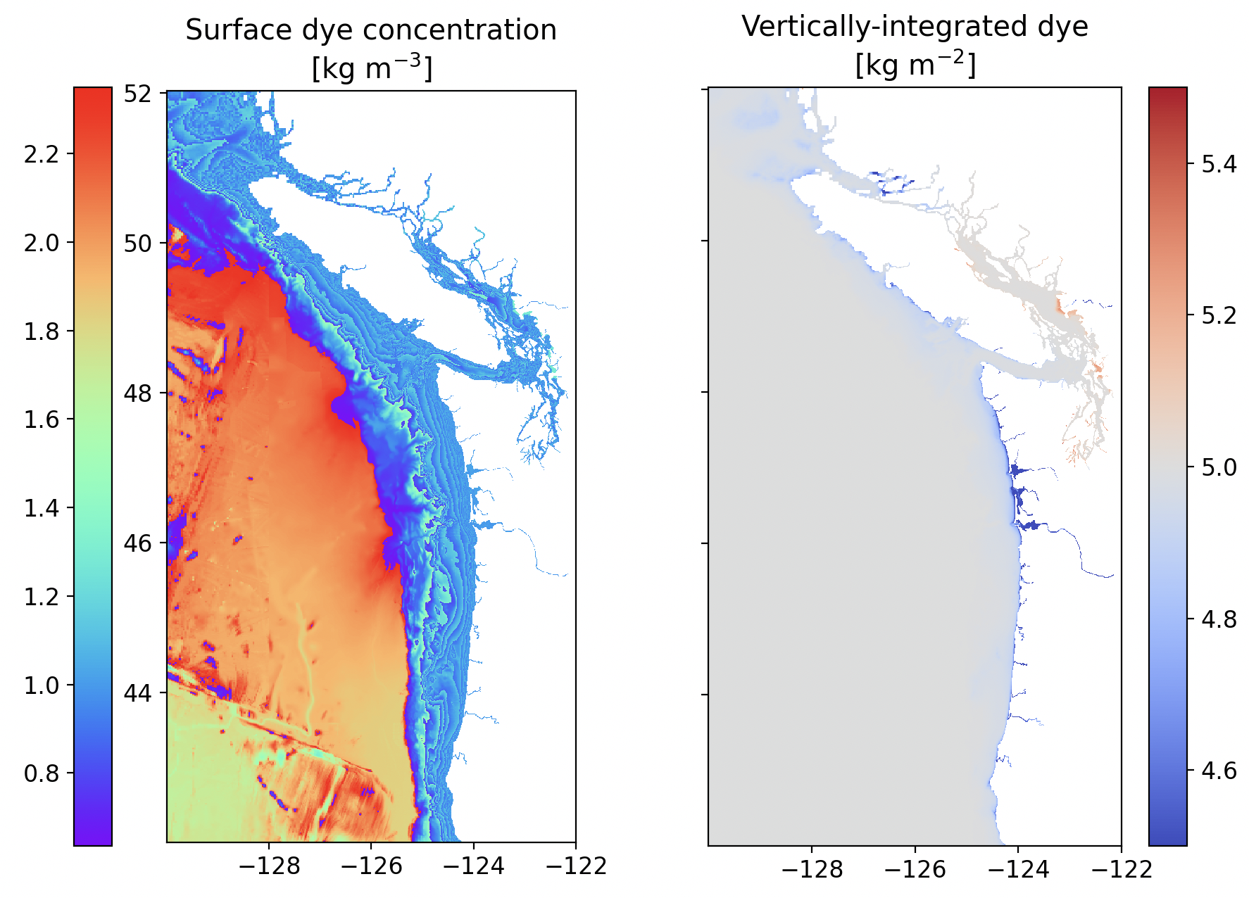
Fig 1. (a) Surface dye concentrations across the model domain. Nominal concentration is 1 kg/m3. (b) Vertically integrated dye concentrations. If correct, this should evaluate to 5 kg/m2 everywhere.
After some debugging last night, I discovered something deeply unsettling: I forgot to account for shifts in water depth due to SSH variability. The “oh shift!” realization is that I based my new dye code on my older legacy code, which also contains the same error.
The most unsettling part of this error is that it remained undiscovered for years. Are there any other errors that I haven’t caught yet? I always test code as I go, but it seems that some bugs can still slip through. Yikes.
The extent of the problem
Paper 1
I somewhat frantically went through the two-layer DO budget code last night. Thankfully, the budget code is mostly based on Jilian’s work– and she properly included SSH shifts in her calculations (thank you Jilian!).
However, the hypoxic volume time series is impacted by the SSH shift bug (Figure 2).
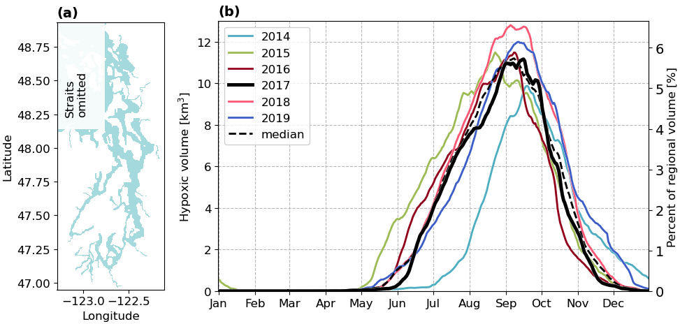
Fig 2. (a) Region over which we integrate (b) Hypoxic volume time series in Puget Sound region
I will need to correct this figure. I do not imagine the plot will change much, but it still needs to be accurate. Now that Kate has taught me how to make masks of Puget Sound, I also thought of adjusting the integration region so we integrate solely within Puget Sound.
Are these corrections something that I need send out immediately, or something I can do in the first round of revisions?
Chapter 2
My SSH shift bug is also affecting the volume integrals I have calculated for the loading/no-loading experiments. Thankfully I caught the bug early enough that I can re-calculate everything before making a poster for Ocean Sciences.
Back to dye
Now that I discovered the SSH shift bug, I was able to correct the surface dye scripts (Figure 3).
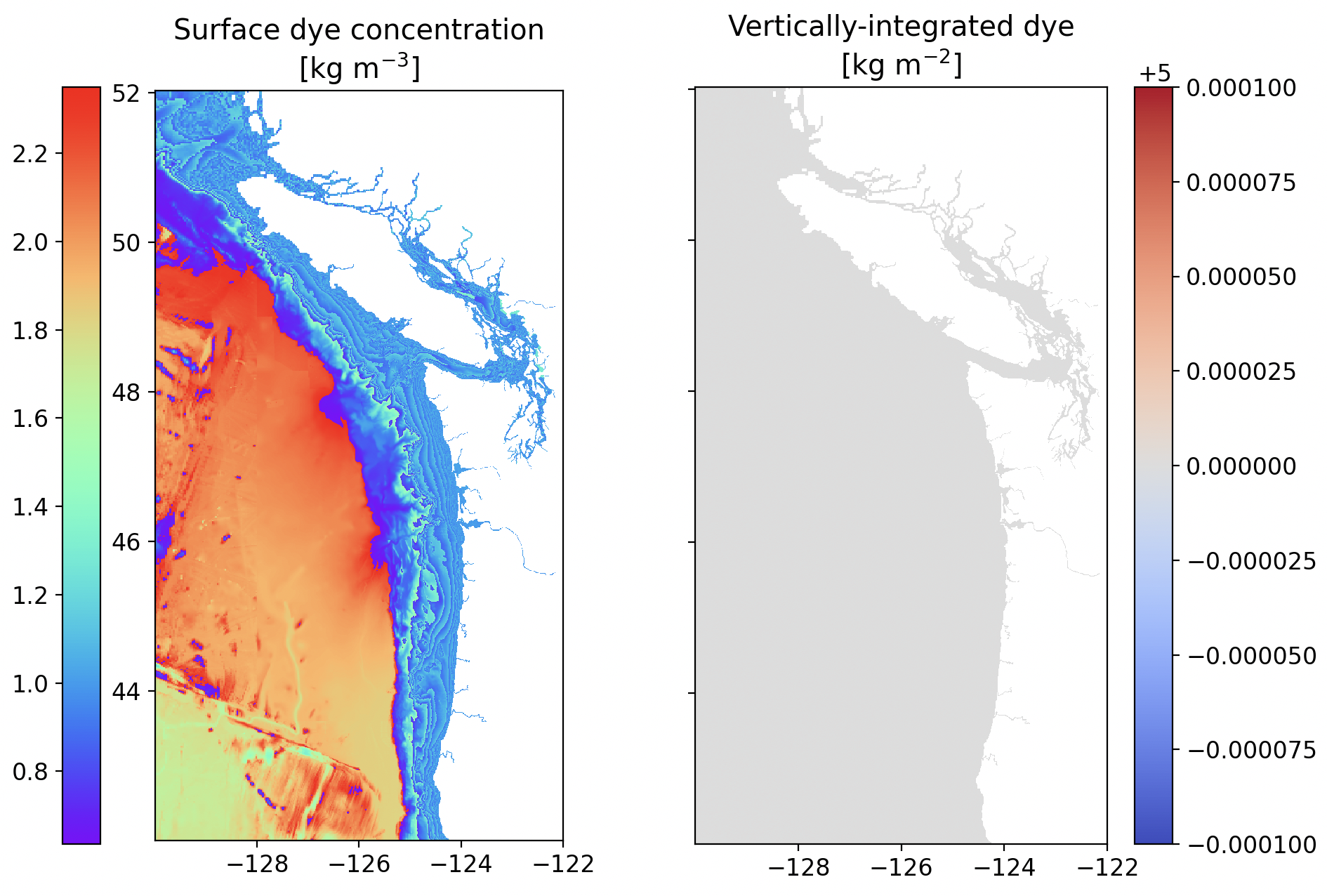
Fig 3. (a) Surface dye concentrations across the model domain. Nominal concentration is 1 kg/m3. (b) Vertically integrated dye concentrations. If correct, this should evaluate to 5 kg/m2 everywhere.
All other forcing and compiling is already set up and ready to go, so I can finally begin running the dye experiments today.
I will also write up a short set of instructions and descriptions for Kate, since she is graciously offering her time to help me run some of these experiments.