Running surface dye experiments
By this point, I have run one successful surface dye experiment. Daily snapshots of vertically-integrated dye concentration in the top 10 m of the water column are shown in the video below.
Fig. 1 Vertically-integrated dye concentration in the top 10 m of the water column. The video is composed of daily snapshots at the start of each simulation day from 2020.02.08 to 2020.02.21. The simulation starts during a spring tide.
Fig. 2 Vertically-integrated dye concentration over the entire water column. The video is composed of daily snapshots at the start of each simulation day from 2020.02.08 to 2020.02.21. The simulation starts during a spring tide.
This blog post covers planned simulation dates, required steps to run surface dye experiments, and details of the dye implementation.
Planned simulation dates
The current plan is to run 8 simulations across the year 2020, each spanning two weeks in length with daily average output. Nominally, we will run during February, May, August, and November. During each month, we will run one simulation that starts during spring tide, and one that starts during neap tide. The run dates are:
- 2020.02.08 - 2020.02.21 (Feb Spring) [Completed; see video above]
- 2020.02.27 - 2020.03.11 (Feb Neap)
- 2020.05.09 - 2020.05.22 (May Spring)
- 2020.05.31 - 2020.06.13 (May Neap)
- 2020.08.18 - 2020.08.31 (Aug Spring)
- 2020.09.06 - 2020.09.19 (Aug Neap)
- 2020.11.16 - 2020.11.29 (Nov Spring)
- 2020.12.09 - 2020.12.22 (Nov Neap)
Run Steps
The run is called cas7_t1d_x11ad. I have already generated all of the forcing files and initial conditions required to run these experiments.
- Compile x11ad on klone. A copy can be found in Aurora’s LO_roms_user/x11ad.
- Make a copy of Aurora’s dot_in/cas7_t1d_x11ad in your LO_user.
- Modify driver_roms00 to use Aurora’s ocean and river forcing, and Parker’s atmospheric and tidal forcing. An example of my driver_roms00 script is in LO_user/driver/driver_roms00_ALdye, with relevant changes around lines 254 - 264. The generate ocean and river forcing are on apogee in /dat1/auroral/LO_output/forcing/cas7
- Using the new driver file, run on klone with 96 cpu-g2 nodes. Launch the run with “newcontinuation.”
Details of Implementation
Header file (compiling ROMS)
The executable is named x11ad. a is for averages, d is for dye. Using x11ab as a template, the following changes were necessary:
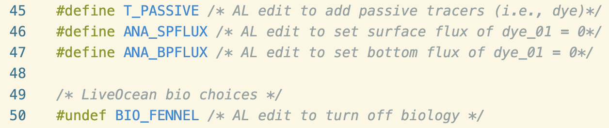
The T_PASSIVE turns on passive tracers, and allows us to use the dye_01 variable. ANA_SPFLUX and ANA_BPFLUX turn on analytical surface and bottom fluxes of tracers, respectively. By default, they are set to zero. Lastly, I undefined BIO_FENNEL to turn off the bio module since we do not need it for this experiment.
Dot_in file for cas7_t1d_x11ad
Using cas7_t1_x11ab as an example, I first deleted bio_Fennel_BLANK.in and commented out all bio code at the end of make_dot_in. I also added a new tiling scheme in make_dot_in to accomodate running on 96 cores.
In BLANK.in, I made the following changes:
- Tell ROMS that we have one passive tracer
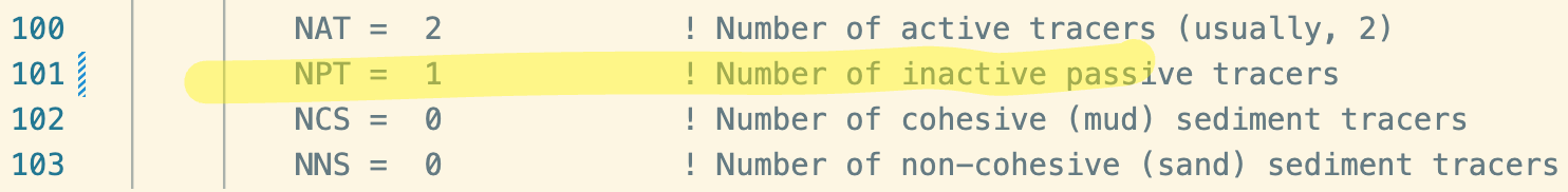
- Add a “F” statement for our tracer since we are not using a sponge

- Add a “T” statement to activate tracer discharge from rivers and WWTPs

- Add “T” statements to turn on nudging to climatology for the new passive tracer


- Write dye_01 to the history files

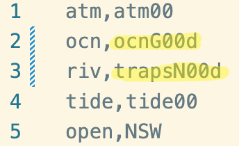
Lastly, in forcing_list.csv, I swapped ocean and river forcing to use new forcing that contains the dye_01 variable:
River forcing
River forcing is trapsN00d. The new river forcing is based on trapsN00, but was modified so that each river and WWTP discharge zero dye_01 concentration.
Ocean forcing
Ocean forcing is ocnG00d. It is based on ocnG00. The new ocean forcing was generated by copying ocean_bry and ocean_clm files from Parker’s existing ocnG00 forcing output. They were modified to add a dye_01 variable, with zero concentration coming in at the open boundaries and nudging to a value of zero at the boundaries.
The script that does this is located here.
Ocean initial conditions
Lastly, I wrote a script to generate a new ocn_ini file based on a pre-existing ocean_his file. The reason that we need to generate initial condition files instead of history files is because ROMS needs to initialize and allocate resources for dye_01, which occurs at the initialization step. If we add dye_01 to a history file and run using continuation, then the dye_01 fields will be flooded with NaNs (I learned this the hard way).
My script uses the structure of an initial conditions files, but the values of a relevant history file, to generate a new initial conditions file. It takes an existing ocn_ini file (that Parker had generated for 2020.10.07), and replaces the fields with values from ocean_his_0002 of cas7_t1_x11ab (the long hindcast). If we wanted to generate intial conditions for 2020.02.08, then the script grabs history files from 2020.02.07. Finally, the script adds a dye_01 variable to the new ocn_ini file with uniform surface dye in the top 5 m of the water column. A visualization of this initial condition can be found at the end of this blog post.
The script that generates this new ocean_ini file can be found here.